About cell and WiFi coverage maps
This topic describes the cell and WiFi coverage maps that OSS-ESPA creates, the method used to create them and drive planning considerations and result verification. When you prepare case analysis evidence using your drive data OSS-ESPA generates cell and WiFi coverage maps which allow you to graphically display the drive test data on the ESPA analysis center screen .
OSS-ESPA supports drive data collected on Gladiator Forensics Autonomous Receiver (GAR) for GSM, UMTS, CDMA, LTE and WiFi. Drive test data is primarily collected while a vehicle is driving on streets, however the streets themselves only represent a small geographical portion of the overall cellular system coverage area. There are many cases when it is beneficial to interpolate the values of the measured quantities in locations where the data was not directly collected. To support this type of interpolation, OSS-ESPA uses a patented proprietary algorithm that generates interpolated measurement based grids and uses them to delineate coverage footprints of target cells, towers and WiFi networks. In OSS-ESPA these coverage footprint outputs can be viewed on the ESPA analysis center screen. There are two types of cell coverage maps: "cell footprint maps" and "signal contour maps". ?Signal contour maps are the individual serving cell's surface maps which are derived from all the received drive data for that serving cell, whereas cell footprint maps are derived from all signal contour maps and show only the areas for each serving cell where it is dominant.
Grids are a two dimensional matrix of measurements used to store surface data. They have a rectangular boundary with a geographical reference where the boundary is divided into smaller equal sized squares called “bins”. Each of these bins stores the measurement of interest. There are many grid generation methods and the method used depends on the application, such as:
- Terrain grids derived from contours to grid algorithm
- Land use grid derived from satellite imagery and other known databases
- Surface grids can be derived from models
- Surface grids can be derived through interpolation of table data
Using grid interpolation, OSS-ESPA interpolates any numeric point data that has been placed on a map and produces a surface grid. An example of measured data and its interpolated grid output are shown in the following graphic:
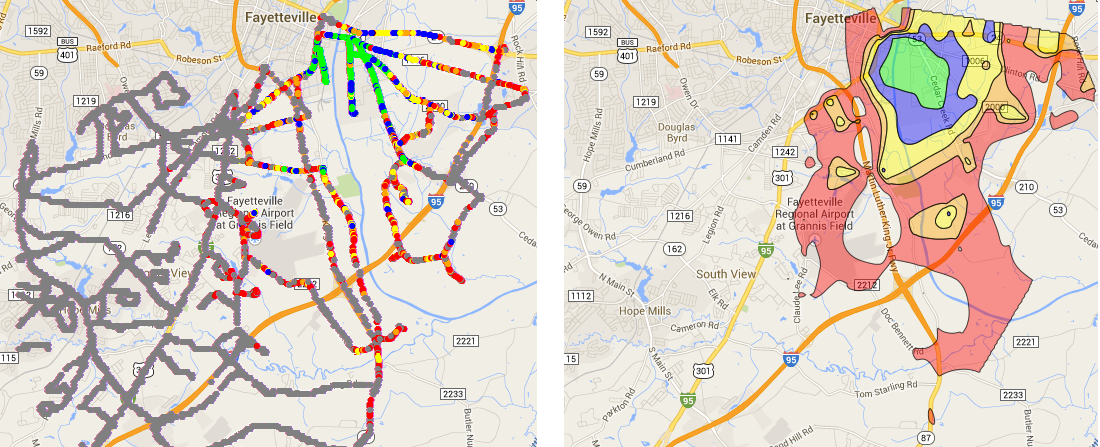
Grid interpolation methods use the measured table data and interpolate this data to fill in the gaps. There are many interpolation methods, such as natural neighbor, rectangular, triangular, and inverse distance weighting. OSS-ESPA uses the natural neighbor interpolation method to produce its cell and WiFi coverage results. This method is best suited for measurements on streets and it is simple to understand and use. The natural neighbor interpolation method builds a network of natural neighbor regions (Voronoi diagram) using the original data. This creates an area of influence for each data point that is used to assign new values to the overlying grid cells.
The Network level outputs folder contains the cell footprint analysis results at the network level, that is it contains the combined results of all cells. For GSM there is only ever one set of results but for other technologies you may have subfolders for each channel/frequency measured during the drive test.
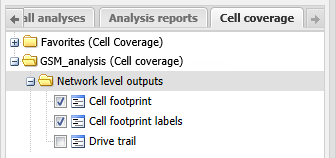
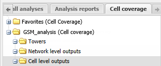
For GSM you only have one folder:
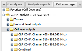
For other technologies you may have multiple subfolders:
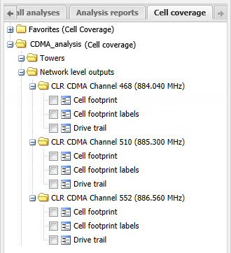
The Network level outputs folder contains three results:
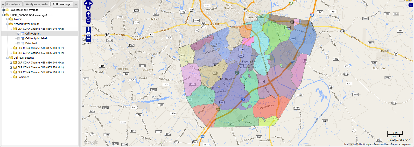
Cell footprint displays on the map the dominant areas of every cell measured during the drive test. The dominant area is the area in which each cell's received signal strength is higher than any other cell and therefore phone calls in that area will most likely use that cell.
Cell footprint labels displays on the map the label obtained from the drive test that identifies each cell, for:
- GSM this is a combination of the Broadcast Channel and the Base Station Identity Code (BCCH_BSIC)
- CDMA this is the Psuedo Noise code (PN)
- UMTS this is the Primary Scrambling code (PSC)
- LTE this is the Physical Cell ID (PCI)
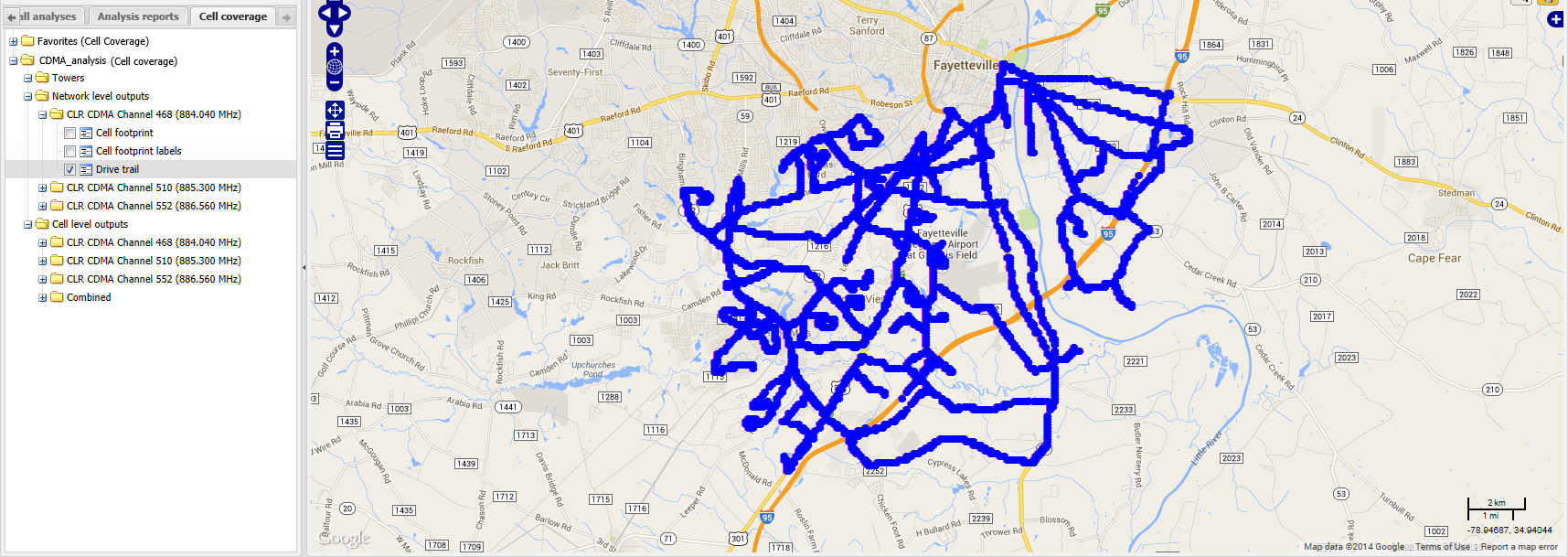
Drive trail displays on the map the route you drove during the drive test.
The Cell level outputs folder contains the cell footprint analysis results at the cell level, that is it contains the individual results of all cells. For GSM there is only ever one set of results but for other technologies you may have subfolders for each channel/frequency measured during the drive test along with a subfolder combining all the channel/frequencies. You should use the combined subfolder if you do not know which channel/frequency was used by the phone. This is the case in most instances as a CDR provides you with the Cell ID but not the channel/frequency. The combined subfolder takes the maximum combined coverage of all frequencies being transmitted from the cell. However if you do know which frequency/channel was used then select the individual channel/frequency.
For GSM you only have one folder:
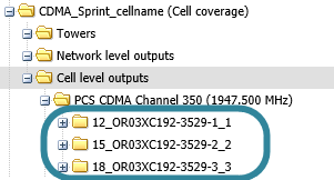
For other technologies you may have multiple subfolders:
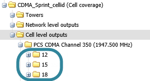
Each of the Cell level outputs folders are named based on what was selected in the L3 output cell matching setting prior to running the cell coverage analysis, so they are either named using: only a numerical identifier assigned by OSS-ESPA, the numerical identifier and the cell ID, or the numerical identifier and the cell name.

Each of the folders contain up to four results:
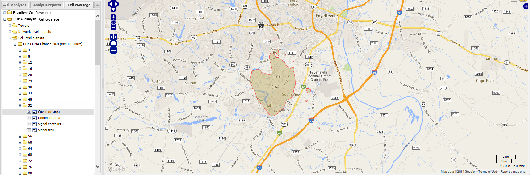
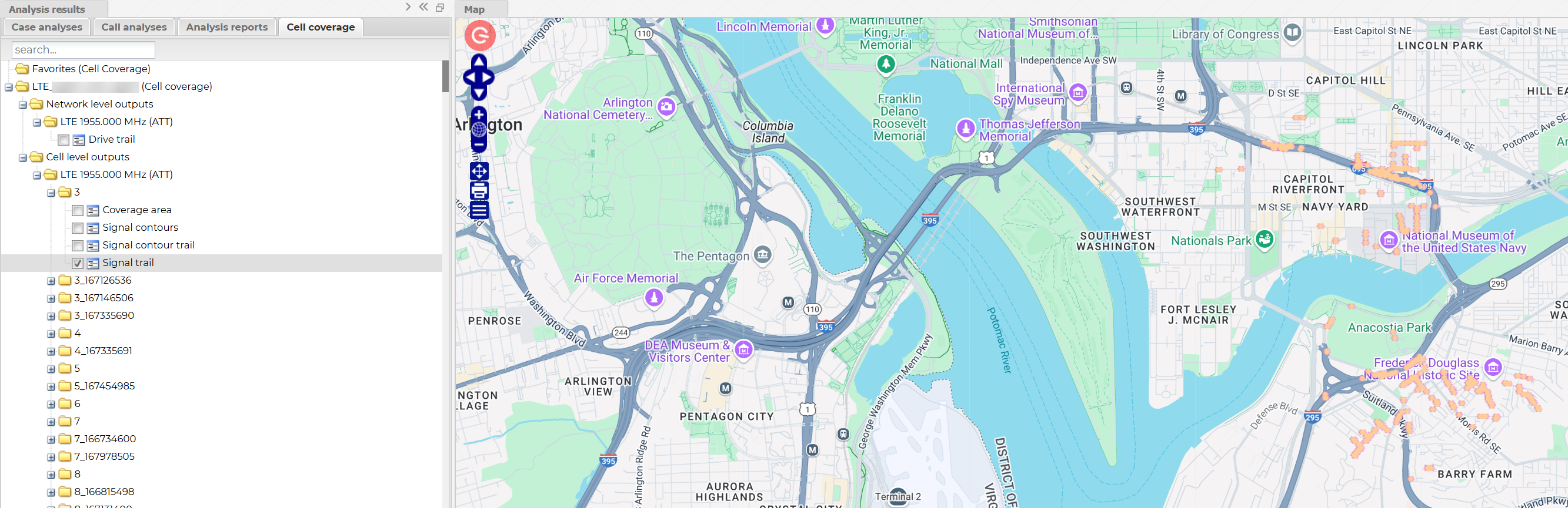
Coverage area displays on the map the area in which the selected cell's signal power level is above the Coverage threshold set in the Cell footprint analysis dialog box. If this output is not displayed for a cell it means that the signal power level for that cell was never above the set threshold. If a suspect has been making multiple phone calls while driving, by selecting the coverage area of each cell that the suspect used it can help you identify the route they were driving.
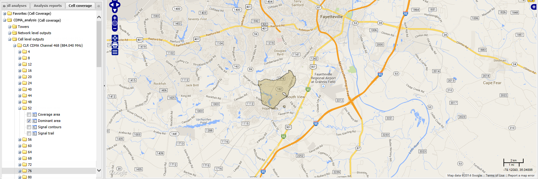
Dominant area displays on the map the area in which the selected cell is dominant. This means that the selected cell's received signal strength is higher than any other cell and therefore phone calls in that area will most likely use that cell. It is this same area that is displayed on the Network level outputs Cell footprint, except at the network level it displays this for every cell. If this output is not displayed it means that another cell with a higher received signal strength was transmitting over the same area.
The dominant areas is only displayed for GSM, UMTS, CDMA and EVDO; it does not display for LTE, NR and IoT.
Signal contours displays on the map the areas in which the selected cell's signal level is in each signal level band. For the selected cell, the signal power level is represented on the map using different colors for each signal level band. The Legend/Filter view displays a key that details the ranges of each signal level band. These signal level bands are defined prior to running your cell footprint analysis in the Cell footprint analysis dialog box.
Signal contours allow you to visualize how the signal degrades geographically (from the green high power signals to red low power signals) as it propagates away from the cell tower. The signal contours clearly identify where the cell's signal cannot reach and therefore where calls physically cannot be made through the selected cell. This is very useful if you are challenging alibi locations.
Signal contours allow you to determine the most likely areas a phone was used. When a phone call occurs in a particular cell the most likely area for the phone's location is in the dominant area, however it may be outside this dominant area. If it is outside the dominant area it is most likely to be in an area where the cell's signal power is higher rather than lower. The signal contours show you the areas covered by each signal level band. This is useful if you need to identify a more specific area, for example if you need to physically search an area for a missing person the signal contours show you which areas have the highest power and therefore they are the more likely search areas. In a search case you should prioritize the dominant area, and then areas covered by the highest signal power.
As mentioned the signal contours most often increase your potential areas of interest from that shown by the dominant area, however there are occasions where it does the opposite and decreases potential areas of interest to less than that of the dominant area. For example if a cell is located near to a large expanse of water, it may show as being dominant over the area of water, however the signal contours may not cover much of the water indicating that the signal power level was so low that a call could not have been in that location even though the cell showed as being dominant over that area.
Signal contour trail displays on the map the route you drove during the drive test. For the selected cell, the signal power level is represented on the map using different colors for each signal level band. The Legend/Filter view displays a key that details the ranges of each signal level band. These signal level bands are defined prior to running your cell footprint analysis in the Cell footprint analysis dialog box. Grey represents areas that you drove where no signal was detected by the selected cell.
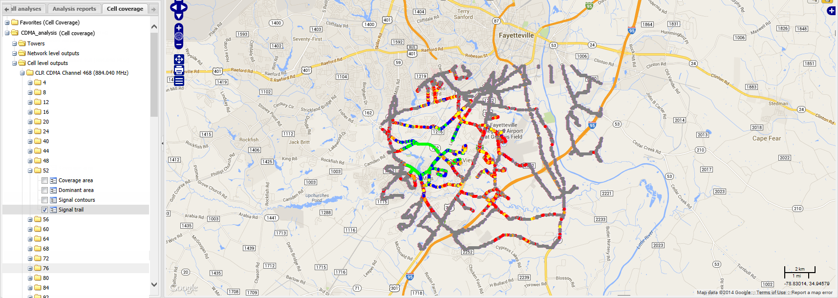
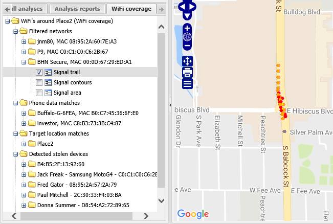
Signal trail displays on the map the route you drove during the drive test where signal was detected. The route is displayed using the same color as the coverage color. There is nothing displayed on the route where no signal was detected, unlike the Signal contour trail which displays grey dots.
The Towers folder contains information relating to the cell towers. The cell tower information that is displayed is from the one you selected in System on the Cell footprint analysis dialog box.
Sites displays on the map all the cell sites that were included in the cell tower data file you selected for your analysis on the Cell footprint analysis dialog box. The cell sites are displayed as colored circles. The color of the circles for each operator can be different if your administrator has configured them with different colors. For example;

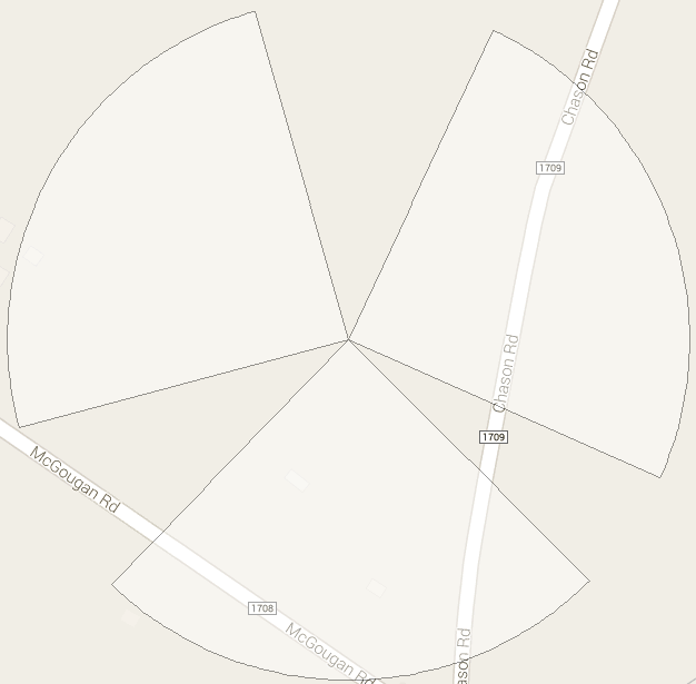
Sectors displays all the sectors that were included in the cell tower data file you selected for your analysis on the Cell footprint analysis dialog box. The sectors display as shown:
Sector labels displays on the map all the cell IDs that were included in the cell tower data file you selected for your analysis on the Cell footprint analysis dialog box. The cell IDs display as shown:
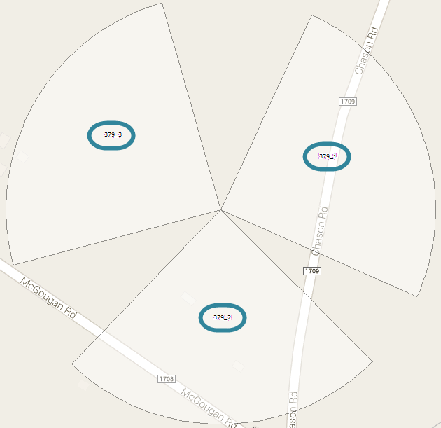
These sector labels are required as they allow you to match the cell footprint results to the CDR data which is not possible using the Cell footprint labels. This is because the drive test results provide the Cell footprint labels using the Layer 1 identifiers (that is, PN, PSC, BSIC/BCCH) and the CDR uses Layer 3 identifiers (that is the Cell ID).
For GSM and UMTS the sector label only consists of one number but for CDMA it consists of the Cell ID and the Sector ID, for example 437-1, 437-2 and 437-3.
Signal area displays on the map the area in which the selected WiFi network's signal power level is above the Coverage threshold set in the WiFi footprint analysis dialog box. If this output is not displayed for a WiFi network it means that the signal power level for that WiFi network was never above the set threshold.
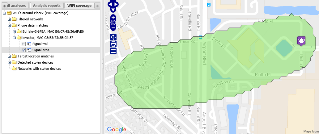
Signal contours displays on the map the areas in which the selected WiFI SSID's signal level is in each signal level band. For the selected WIFi SSID, the signal power level is represented on the map using different colors for each signal level band. The Legend/Filter view displays a key that details the ranges of each signal level band. These signal level bands are defined prior to running your WiFi footprint analysis on the WiFi footprint analysis dialog box.
Signal contours allow you to visualize how the signal degrades geographically (from the green high power signals to red low power signals) as it propagates away from the WiFi network. The signal contours clearly identify where the WiFI network's signal cannot reach and therefore where calls physically cannot be made through the selected WiFi network. This is very useful if you are challenging alibi locations.
Signal trail displays on the map the route you drove during the drive test. For the selected WiFi network, the signal power level is represented on the map using different colors for each signal level band. The Legend/Filter view displays a key that details the ranges of each signal level band. These signal level bands are defined prior to running your WiFi footprint analysis in the WiFi footprint analysis dialog box. Grey represents areas that you drove where no signal was detected by the selected WiFi network.
There are a number of points you should consider prior to your drive, and then after your drive is completed you should verify the results.
Poor drive planning and insufficient samples can cause inaccurate results therefore to minimize inaccuracies you should plan your drive by considering the following:
- Select the drive area on the ESPA analysis center using the polygon tool then export your drive area details into MapPoint. For further information on how to do this refer to Selecting your drive area.
- It is recommended that the scanner you use is the Gladiator Forensic's GAR unit.
- Identify which operators and technologies you require to capture during the drive test.
- View the cell footprint map in the ESPA analysis center screen and check for cells with missing output, that is, verify that coverage exists for each target cell and if coverage does not exist around the cell then redrive the areas around the cell.
-
Analyze the cell level Signal trail and Coverage area together to verify that you have driven a sufficient number of streets within the cell's coverage area.